MH370 Flight Simulation of Path Offset Scenarios

2015/05/10 Duncan

MH370 Flight Simulation of
Path Offset Scenarios

Geoff Hyman
2015 May 10
Updated May 12

1. Background and Summary

This note seeks to contribute to a continuing investigation (references [1], [2], [3]) of scenarios describing the period between last radar contact of MH370 and its final descent. The simulations were conducted using variant BSMv7-10-5_GH of a flight model by Barry Martin which may be downloaded by clicking here or here (warning: the download is 20.9 MB; for further information on Barry Martin’s MH370 flight models, see this webpage and this post and also this post and indeed this post too).

The scope of the model employed is sufficient to include a path offset near NILAM, associated with an increase in altitude, as well the final major turn (FMT). All turns are specified in terms of circular arcs with constant rates of turn. The increase in altitude is specified to be at a constant rate of climb (RoC). The program supports a temporal resolution of 15 seconds, proximity calculations of flight paths from designated waypoints, outputs relating to turn characteristics, plus a range of error criteria which may be used either to compare the statistical fit of alternative flightpath or to estimate selected unknown flight parameters.

The principal finding from the current investigation is that the most probable scenario is an offset path during the late middle game which did not continue beyond the FMT. Implications in terms of human and system factors are discussed.

The implied zero altitude locations from all of the tests are close to the published nominal IG September 2014 location [4], given as 37.5S, 89.2E. This report does not deal with estimated endpoint coordinates, as this requires a more detailed simulation of the final descent [5].

2. Initial Conditions, Key Outputs and Estimates

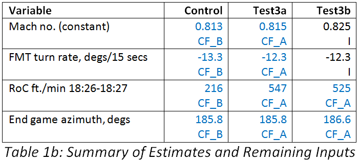
Table 1a shows the major input assumptions and principal model outputs. The second column in Table 1a, labelled ‘type’, adopts the abbreviations:
I: Input values/initial conditions
O: Values computed explicitly from the flightpath model

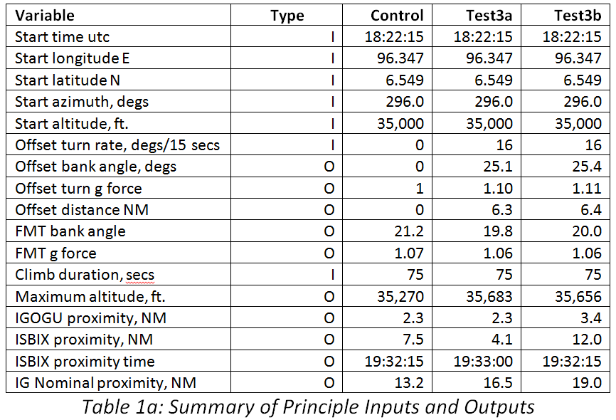
For some of the variables, values were estimated by minimisation of an error cost function (CF), using an approach which varied between the modelled scenarios, as specified in Table 1b.

GHtable1b

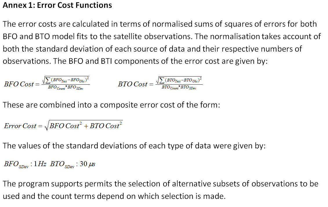
The value of the error cost function depends on both the underlying uncertainty in their true values and on which observations are selected for error cost minimisation. Further details of the specification of the error cost function are given in Annex 1 and in Section 4 below.

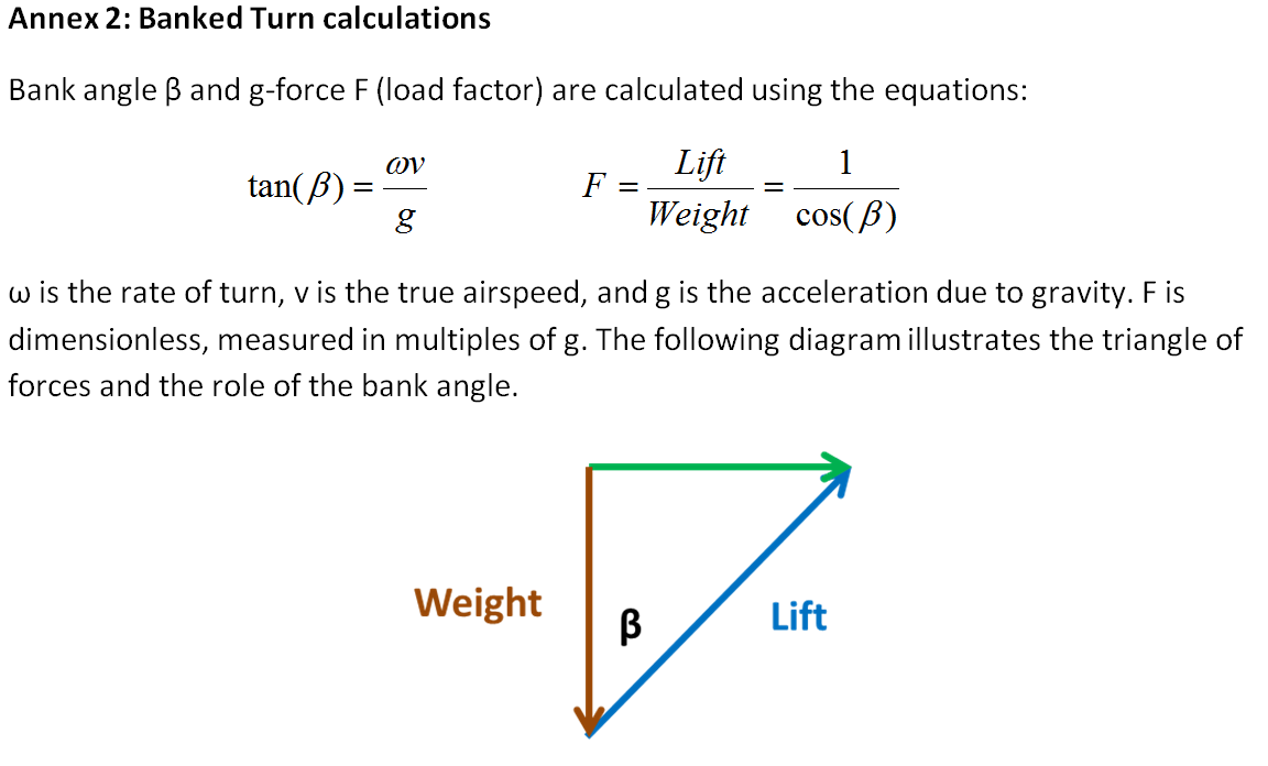
For the scenarios reported here, the start azimuth was assumed to be at the N571 alignment of 296 degrees (measured through east from true north). To conform to limits of lateral navigation, all turns were constrained to be within a bank angle that did not exceed approximately 25 degrees. The corresponding g force experienced would therefore not exceed 10% above normal gravity. The equations used for the banked turn calculations are given in Annex 2. The FMT was constrained to terminate by 18:40 and to be executed within a period of just over two minutes.

Each scenario used a different approach to select which of the unknowns were estimated, and which observations were used to estimate them. In Table 1b, CM_A and CM_B refer to different subsets of observations employed for cost minimisation, as detailed in Table 2.

It can be noted that the estimated Mach numbers were similar in the Control scenario and Test 3a. For Test 3b a slightly higher value was input, to produce an offset which continues into the end-game (i.e. post-FMT). The estimated climb rates (RoC) were moderate but varied between scenarios, giving increases in altitude of over 500 feet for Tests 3a and 3b, but of less than 220 feet for the Control scenario.

The proximity (minimum distance) from the nominal IG September 2014 location were all computed assuming an altitude of zero (i.e. assuming that the 7th ping ring is located close to, or at, sea level; see this recent post). However, the waypoint and offset distances were calculated by finding the minimum distances of the offset paths from a reference location on the Control path, at a common altitude of 35,000 feet.

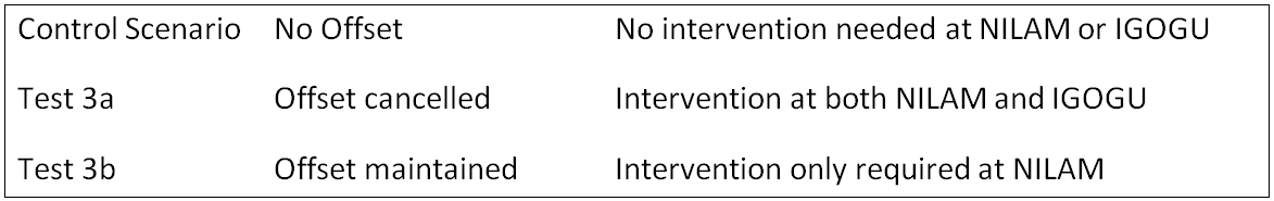
3. Three Scenarios, a Suggested Interpretation and a Disclaimer

The selection of the three scenarios presented arose from a suggestion made by Sid Bennett, who set out clearly how they might be expected to operate. His contribution is gratefully acknowledged. Their suggested interpretation arises from discussions with Barry Martin, who created the program being used for flight path analysis and whose contribution is also gratefully acknowledged. Any errors or misunderstanding in this report are entirely my own. Two short extracts from Sid’s proposals are given in italics below.

The Control scenario represents a flight path with no offset. Its statistical support requires setting aside the 175 Hz BFO observation at 18:27. This type of scenario may have been implicit when the IG presented its September 2014 report.

Test 3a assumes that the 18:27 BFO observation is valid and results in an offset path, commencing shortly after the NILAM waypoint. This is an example of the type of scenario which was examined in [2] and in recent discussions within the IG. It transpires that, under the specified modelling assumptions for this test, the calculated path offset was not maintained after the IGOGU waypoint (i.e. there was ‘offset cancellation’). It seems that such a scenario is unlikely to be a result of the automatic operation of the flight management system (FMS), which would require the final major turn to exceed 135 degrees. Instead it would appear to require active human intervention near IGOGU:

“… the pilot cancels the offset either sometime before IGOGU or sometime after IGOGU, but before ISBIX. In the end, both options result in the plane flying the radial between IGOGU and ISBIX…” (Sid Bennett)

This may be contrasted with Test 3b, a path for which the path offset is maintained beyond the FMT:

“… After continuing the offset track south of IGOGU, the track continues parallel to the radial joining IGOGU and ISBIX as a geodesic until abreast of ISBIX and then continues as a lox [loxodrome] without changing the azimuth…” (Sid Bennett)

This scenario could, in theory, have been flown by the FMS, so it would not have required human intervention.

The formulation of these alternatives is particularly interesting. Assuming that they characterise the possibilities we might proceed by a process of elimination. First, if we were convinced that an offset had occurred, this would eliminate the Control scenario. The initial offset would have required active human intervention at about 18:27. If it were impossible in practice for the satellite data to discriminate between offset continuation and offset cancellation, it would then be difficult to determine if human intervention had or had not continued. Alternatively if one or other of the offset scenarios (Test 3a, Test 3b) could be eliminated then this ambiguity would be resolved. The following interpretations of the scenarios are proposed:

We will assess the comparative weight of evidence in favour of each of these cases.

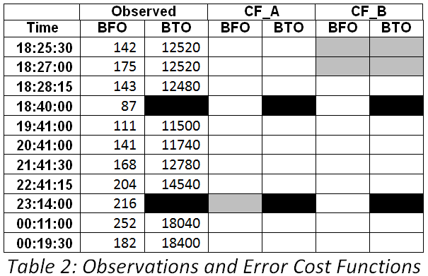
4. Specification of the Cost Functions in terms of their constituent observations

Table 2 reports the BFO and BTO observations which were used in each of the error cost functions. The grey cells indicate observations which were excluded from individual cost functions. The black cells show where no BTO observations were available.

For CF_A the BFO observation at 23:14:00 was excluded. This cost function was used to estimate unknowns in Tests 3a and 3b. For CF_B the observations (both BFO and BTO) at 18:25:30 and at 18:27:00 were excluded. This was used for the estimation of unknowns in the control scenario. The program automatically excludes all observations which occurred prior to the common start time of the scenarios of 18:22:15.

5. The Appearances of the Flight Paths for the Three Scenarios

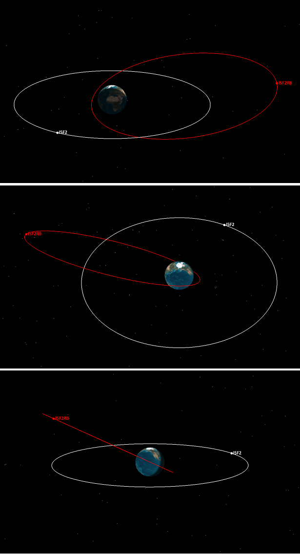
Figure 1 shows the three flight paths over the full simulation period. At this resolution two paths (the red path is for the Control scenario, and blue path for Test3a) appear indistinguishable. They both pass within 20 nautical miles (NM) to the east of the nominal IG September 2014 location (37.5S, 89.2E; shown by the red X marker on the 7th ping ring). The dashed green Test 3b path passes within 20 NM to the west of the nominal IG September 2014 location.

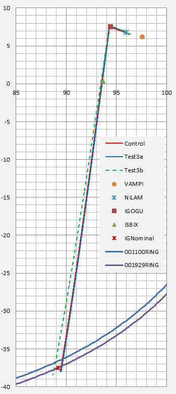
Figure 1: The Three Flightpaths in relation to the
Nominal IG September 2014 location

Figure 2 shows the paths in the vicinity of the ISBIX waypoint. The closest proximity between the Test 3a path and ISBIX is 4 NM, while the closest proximity of the Test 3b path to ISBIX is 12 NM, a difference of 8 NM.

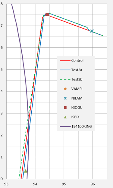
Figure 2: The Three Flightpaths in relation to the ISBIX waypoint

If we refer back to Table 1a we may note that the middle-game offset distance for both of these paths is between 6 and 7 NM. The difference of 8 NM distance from ISBIX is therefore sufficient to discriminate between a flightpath for which the offset is cancelled and one for which it is maintained.

The intersection of the Test3b path and the Control path, at a latitude near 5.7 degrees north, is also apparent in Figure 2.

In Figure 3, the red Control path exhibits no offset. Test 3a and 3b (dashed) have offsets starting near the NILAM waypoint, at distances of slightly over 6 NM from the Control path.

The early end-game path for the Control scenario commences to the west of the Test 3a path. This is unsurprising because, during the late middle-game, the offset paths are longer than the Control path. The Control path has the same speed as Test 3a, so it can proceed further west in the same elapsed time as the Test 3a path. The same check could not be used to compare the Control path with Test 3b, as the latter has a slightly higher speed.

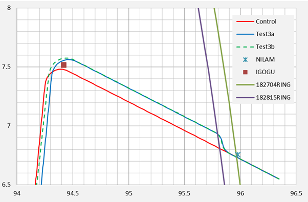
Figure 3: The Three Flight Paths in relation to
NILAM, IGOGU and the Final Major Turn

6. Error Analysis

Table 3 shows the BFO and BTO errors for each of the three scenarios. Values in excess of three standard deviations have been highlighted in yellow. Two of these errors apply to all three scenarios: the BFO errors at 18:25:30 and 23:14:00. At 23:14 similar errors have been noted for examined previously scenarios [2] and these could be either intrinsic to the observations, or due to unknown factors which have not been accommodated in any of the modelled scenarios. Previous simulations support the view that the 18:25:30 errors are correlated with the value of the middle-game azimuth.

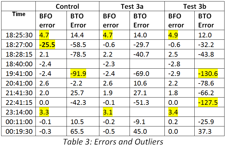
Next we look at those errors which help us discriminate between the current scenarios (Control, Test 3a, Test 3b). By far the largest error is for the BFO observation of 175 Hz at 18:27 when compared with the Control scenario. The best available explanation that we currently have for this is that an offset turn had occurred. This error is not present in the other two scenarios. Comparing Test 3a with Test 3b we note that the latter has two large BTO errors: at 19:41 and 22:41:15. For Test 3a, while errors are also present at these times they are of a much smaller magnitude. A broader statistical assessment is of interest.

Table 4 below reports the values of the error cost functions and their BFO and BTO constituents.

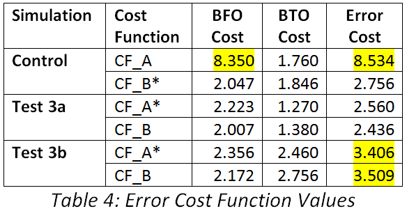
The second column in Table 4 indicates the cost function being reported, with an asterisk (*) being used to indicate which of them was used to estimate the unknowns. Test 3a performed best for both cost functions, and also for their BFO and BTO components.

The worst values are highlighted in yellow. The Control scenario performed the worst for CF_A, while Test 3b performed the worst for CF_B.

Pairs of scenarios can be compared by treating the error costs as standard normal deviates and calculating odds ratios. On this basis under cost function A (CF_A), Test 3a would have ten times higher a likelihood than Test 3b; and under cost function B (CF_B), Test 3a would have twenty times the likelihood. From either view, it would be reasonable to reject Test 3b (the continuing offset scenario). It remains a challenge to construct continuing offset scenarios which achieve substantially better performance with respect to the same observations.

The comparative odds for each of the test paths (3a, 3b) can also be compared with the Control scenario. Clearly under CF_A the Control scenario would be very strongly rejected, so it suffices to restrict attention to CF_B. On this basis the offset cancellation scenario (Test 3a) is only twice as likely as the Control scenario. Therefore, if the null hypothesis was the Control (no offset) scenario, it could not be rejected with a high degree of confidence.

We appear to be faced with a realistic choice only between either the no offset scenario (the Control scenario) or the offset cancellation scenario (Test 3a). Which of them is correct depends on the validity of the observations near 18:27 UTC. If they are considered valid then we have eliminated everything but the offset cancellation scenario.

7. Implications of Findings for Likely Scenarios and Human versus System Factors

In discussing the full set of findings we needed to discuss alternative stances with respect to the satellite observations at 18:27 (cf. the apparently-large BFO at that time). First, we will adopt a sceptical view and exclude them from consideration. A scenario without an offset is simpler as it has fewer degrees of freedom. An application of Occam’s razor would thereby make the no offset (Control) scenario the null hypothesis. On the sceptical view, this could not be rejected with a reasonable degree of confidence and the case for an offset would be weak, even though it appears as a slightly more likely alternative. Without an offset no human intervention would be implied during the late middle-game, and again this would seem to be a simpler interpretation of events. However its simplicity also makes it easier to falsify.

Next, we include the 18:27 observations, accepting them as valid. The case for an offset now becomes extremely strong and the issue is primarily whether or not it was cancelled. The scenarios presented here support the view that offset cancellation is the more likely scenario. The implication would be that human intervention had probably occurred, and that it had continued at least until the vicinity of IGOGU.

Conclusions concerning the continuation of human intervention beyond ISBIX, until the final descent, are outside the scope of this report.

References

[1] Bennett S. and Hyman G. Further Studies on the Path of MH370: Turn Time and Final Azimuth. MH370 Independent Group, March 2015.

[2] Hyman G., Middle game uncertainties in azimuth, with implications for the MH370 endpoint. MH370 Independent Group, April/May 2015.

[3] Exner M., Godfrey R. and Bennett S. The Timing of the MH370 Final Major Turn. Independent Group, March 2015.

[4] Steel D., MH370 Search Area Recommendation. MH370 Independent Group, September 2014

[5] Anderson B. The Last 15 minutes of Flight of MH370. MH370 Independent Group, April 2015.

Astronomy & Space Science, Orbital Debris

The Orbital Debris Collision Hazard for Proposed Satellite Constellations

2015/04/30 Duncan

The Orbital Debris Collision Hazard for
Proposed Satellite Constellations

Duncan Steel
2015 April 30

Introduction

In my first post here on the calculation of orbital debris collision hazards I wrote the following in connection with reported plans to insert constellations of satellites into low-Earth orbit (LEO), in the following case at altitude 800 km:

“If these enhancement factors are of the correct order, then the collision probability attains a value of around 5 × 10^-3 /m²/year, implying a lifetime of about 200 years against such collisions with orbital debris. This indicates that there is cause for concern: insert 200 satellites into such orbits and you should expect to lose about one per year initially, but then the loss rate would escalate because the debris from the satellites that have been smashed will then pose a much higher collision risk to the remaining satellites occupying the same orbits (in terms of a, e, i). This ‘self-collisional’ aspect of the debris collision hazard I highlighted in the early 1990s.”

The enhancement factors in question are those that elevate the collision probability for any planned satellite above the value I had calculated on the basis of the orbits of the 16,167 objects listed in the Satellite Situation Report in early April. These factors may be summarised as follows: (a) The lack of available orbits for objects that are CLASSIFIED, this potentially increasing the collision probability by 25 to 50 per cent; (b) An increase by a factor of two or three in the collision probability due to the finite sizes of tracked objects compared to the one-square-metre spherical test satellite assumed in my calculations (with the potential impactors being taken to be infinitesimally small); and (c) The overall collision probabilities being higher perhaps by a factor of a hundred due to the large population of orbiting debris produced by fragmentation events that is smaller than the (approximately) 10 cm size limit for tracking from the ground by optical or radar means but nevertheless large enough to cause catastrophic damage to a functioning satellite in a hypervelocity impact.

Herein I consider in more detail two mooted satellite constellations, intended to deliver internet access to the entire globe, and assess the orbital debris collision hazard that they will face; and also the hazard that they would pose to themselves and other orbiting platforms should the plans go ahead.

Proposed internet satellite constellations

Several distinct satellite constellations have been proposed and are apparently undergoing development, although definitive information is sparse. As an initial illustrative example I will describe WorldVu, a proposal stemming from former employees of Google although subsequently spun off into a new company and rebranded as OneWeb. The original WorldVu plan apparently involved a constellation of 360 satellites in total, 180 each at altitudes of 800 and 950 km, and all having an inclination of 88.2 degrees. At each altitude the 180 satellites would be arranged in nine orbital planes each containing twenty satellites. Shown below is a visualization of just the 180 satellites at altitude 950 km, with the blue access cones beneath each satellite indicating the coverage of Earth’s surface subject to a limitation of the elevation angle from ground to satellite being at least 25 degrees (this being a conceivable limit for ground station access to each satellite).

Graphic above: A Strawman satellite constellation of 180 platforms in polar orbits. A movie showing the movement of these satellites in orbit is available for download from here (14.4MB).

My previous posts on the LEO debris collision hazard (here and here) have shown that the collision probability against tracked orbiting objects is particularly high for altitudes 800-1000 km, most specifically for any proposed satellite in a polar orbit (inclinations 80-100 degrees).

Perhaps in recognition of the crowded and congested nature of geocentric space at such altitudes, more recent (i.e. in 2015) proposed satellite constellations have involved slightly higher altitudes, at 1100 km and 1200 km. The two specific constellations that I consider here may be summarised as follows.

OneWeb: 648 (or possibly 700) satellites at altitude 1200 km; individual satellite masses of order 125-200 kg; strategy to evolve to a second-generation constellation of 2,400 satellites.
SpaceX: 4,025 satellites at altitude 1100 km; individual satellite masses 200-300 kg.

Whether or not the above basic information is realistic or not, and whether or not either or both of these proposals go ahead, the two provide pertinent input data for a consideration of the orbital debris hazard that such constellations will face.

Collision probability calculations

I have derived collision probabilities between test satellites and my list of 16,167 tracked orbiting objects as described previously. Although the satellite altitudes (i.e. 1100 and 1200 km) are known, I do not know for certain the proposed inclinations. The previously-promoted WorldVu plan was for an inclination of 88.2 degrees. A graphic from OneWeb shown immediately below indicates polar orbits. Sun-synchronous orbits for altitudes of around 1110-1200 km require an inclination close to 100 degrees. In view of the above I have performed collision probability calculations for those two inclinations, 88.2 and 100 degrees. Note that this means that I have also assumed that the SpaceX constellation would be in polar orbits (and it might well be that lower-inclination orbits would be chosen so as to provide better coverage of low-latitude rather than polar ground locations).

Above: The proposed OneWeb satellite constellation’s orbits and ground coverage (source: OneWeb website).

In Figure 1 are shown the collision probabilities for test satellites in circular orbits in 50 km steps between altitudes 650 and 2000 km, for the two inclinations discussed above. Purely on the basis of minimising the debris impact risk it is clear that it would be wise to avoid altitudes below 1000 km or even 1050 km.

Figure 1: Collision probabilities against all tracked objects in the publicly-available Satellite Situation Report as a function of altitude for circular test orbits and for two different near-polar inclinations; a spherical test satellite of cross-sectional area one square metre is used, and all possible impactors (the tracked objects) are taken to be infinitesimally small (i.e. the mutual collision cross-section is assumed to be one square metre in every case).

The form of Figure 1 might, in isolation, be thought to imply that there are comparatively few objects whose orbits take them above 1,000 km altitude, and indeed it has been reported in the media that this is one reason for the SpaceX choice of an altitude of 1100 km. However, this is not the case: there are many tracked objects in orbits well above 1000 km. In Figure 2 I plot the numbers of tracked objects with orbits that cross each of the discrete altitudes in Figure 1. Whilst that plot peaks at 850 km with just over 5,000 tracked objects, there are still about 3,000 tracked objects crossing 1100-1200 km, and over 2,000 objects right the way up to altitude 2000 km.

In view of the information in Figure 2 it might seem surprising that the collision probabilities as shown in Figure 1 drop rather quickly at altitudes above 1000 km. The lesson to be learned from this is that mere numbers of objects do not provide a reliable indication of the collision risk: their orbits (and especially their inclinations) greatly affect the formal collision probabilities. It happens that polar orbiters have disproportionately high collision probabilities (with extreme likely impact speeds), and most polar orbiters (e.g. in sun-synchronous orbits) circuit our planet at altitudes below 1000 km.

Figure 2: Numbers of tracked objects with orbital paths crossing discrete altitudes between 650 and 2,000 km.

In order to move from a collision probability per square metre per year (as in Figure 1) to a collision probability for specific satellites we need to have some information regarding their size. Although ballpark masses have been stated above for individual satellites in the proposed OneWeb and SpaceX constellations, specific linear dimensions are not known (at least by me!). The graphic below shows an artist’s representation of a OneWeb satellite, and that I have used to estimate that a size of about 5 × 1 × 1 metres is of the correct order.

Above: Representation of a OneWeb satellite in orbit
(source: OneWeb website).

During each orbit the satellites will rotate their solar panels so as to maintain their direction towards the Sun, and this will have the effect of ‘averaging out’ the cross section with regard to debris approach directions. In view of that I will adopt a characteristic cross-section of three square metres for the OneWeb satellites.

Media reports of the masses and planned capabilities of the SpaceX constellation satellites indicate that these may well be larger. For these I will adopt a characteristic cross-section of five square metres.

Regardless of the choice of inclination (88.2 or 100 degrees) the collision probabilities in Figure 1 at altitudes of 1100 and 1200 km are approximately 3 × 10^-6 and 2 × 10^-6 respectively, per square metre per year. These lead to the following estimates for the collision probabilities, when the cross-sectional areas of the satellites are included:

OneWeb satellites: 6 × 10^-6per year

SpaceX satellites: 1.5 × 10^-5per year

It is emphasized that these values should be considered to be lower limits on the orbital collision probabilities, due to factors that have been previously mentioned: (i) There is no allowance for CLASSIFIED orbiting objects; (ii) The finite (often large) sizes of other objects will enhance the collision cross-sections by an average of perhaps two or three; (iii) No allowance has been made for small (less than 10 cm) untracked debris items, and these can increase the collision risk by a large amount; note also that the capability to detect and track small debris items falls off with altitude, given that the US DoD sensors are ground-based.

I would have difficulty in making a case for overall enhancements in the collision probabilities due to the preceding considerations being less than by a factor of ten, and quite likely the true enhancement is by 20 to 50. It may only be through statistics of satellite losses that we will be able to obtain a true assessment of the hazard, or else satellite-borne sensors counting the frequency of near-misses by small orbiting debris (plus natural meteoroids).

If one adopts an enhancement by only a factor of ten, perhaps dominated by 1-10 cm untracked debris from disintegrations such as the Chinese ASAT demonstration in 2007 and that of DMSP-F13 just less than three months ago (see my notes in this post), the catastrophic collision probabilities against orbiting debris become:

OneWeb satellites: 6 × 10^-5per year

SpaceX satellites: 1.5 × 10^-4per year

(Note that although the two satellite disintegrations mentioned above occurred at around 850 km, tracked debris fragments from them have attained apogees crossing the altitudes of the above two proposed satellite constellations; and smaller, untracked debris items generally have larger relative speeds, making them more likely to attain higher apogees. I also note that at this stage the cause of the observed disintegration of DMSP-F13 is unknown, and it might well have been due to an impact by a fragment of the Chinese ASAT target, Fengyun-1C.)

Next I multiply the above probabilities by the number of satellites in each proposed constellation (648 and 4,025 respectively), to obtain an estimate of the loss rates:

OneWeb constellation: 0.04 per year
(one catastrophic collision per 25 years)

SpaceX constellation: 0.6 per year
(one catastrophic collision per 20 months)

A note here on collision speeds: the most likely impact speeds for mutual collisions between polar orbiters at these altitudes (1100-1200 km) are above 14 km/sec.

Implications

The above estimated satellite loss rates due to debris collisions might be considered to be tolerable, but there are other implications. The most important matter, which stems directly from the sorts of calculations performed here, is that any satellite (or other associated object such as a rocket body) in a constellation that suffers a catastrophic fragmentation event immediately elevates the collision hazard for all other satellites that remain in similar orbits. Essentially, the collision probability between two orbiting objects goes up markedly when they have similar orbits, in terms of their perigee/apogee altitudes and inclinations (or a, e, i).

As an example, consider one satellite in the proposed SpaceX constellation which undergoes a disintegration due to being hit by some random piece of orbiting debris. The figures above indicate that such an event is to be expected within the first two years of the deployment of the proposed constellation (and by the time that the constellation is deployed the orbital debris hazard will certainly be worse, not better). Let us assume that the satellite dry mass is 250 kg. Observations of the mass distributions of objects fragmenting in orbit, and indeed deliberate (chemical) explosions of spare satellites in laboratories, indicate that more than 10,000 fragments with masses above 1 gram are to be expected, and each will be moving on an orbit distinct from the parent satellite but nevertheless on quite a similar path. Each of those fragments now poses an impact hazard to all other satellites in the constellation: they are no longer subject to station-keeping, and they are no longer moving in step with the functioning satellites.

(There is an entirely different way of looking at this, that astrophysicists will likely understand. To first order one may say that if there are n satellites in a constellation then the collision hazard they pose to themselves goes up as n² rather than n.)

Assuming an original satellite orbit to be circular at 1100 km, and the debris initially to have perigee and apogee heights spread a few kilometres above and below that, the collision probability for each fragment with each of the other satellites is found to be about 5 × 10^-7per year. For 10,000 fragments capable of colliding with 4,000 functioning satellites the collision rate is then:

5 × 10^-7 × 10,000 × 4,000 = 20 per year

What happens, of course, is not that twenty satellites per year are lost, but rather a rapid cascade occurs with a proliferation of debris in similar orbits obliterating all functioning satellites and leaving that region of LEO unusable for a very long time. This is the Kessler syndrome writ large.

Final comments

Although in this series of posts on orbital debris I have been making use broadly of test satellites assumed to be spherical, that is a non-necessary simplifying assumption. In fact it is possible to derive face-dependent impact probabilities and indeed impactor speed distributions for satellites that maintain their orientations during an orbit, and I not only have software to do this, but have exercised it in the past. Most of my results from the use of that software has not been published, either here or elsewhere; I am intending to prepare other posts for publication here, illustrating the sorts of understandings that can be derived (and it is only through understanding a problem that we can equip ourselves with the wisdom to act and react in certain ways).

There are at least two good reasons to make use of such software when planning future satellites. The first is so that a proper assessment of the orbital debris hazard can be made, making use of the real size and shape of the satellite (including its solar panels) rather than an assumed spherical form, as here. The second reason is that, at least for very small debris items (and indeed meteoroids and interplanetary dust), knowledge of the most likely arrival directions and speeds would enable appropriate shielding to be installed, and also the arrangement of the more sensitive parts of the satellite to be planned so as to minimise the overall mission risk. One cannot entirely obviate the orbital debris collision risk, but one can make judicious decisions on how to minimise it once one is well-informed.

Astronomy & Space Science, Orbital Debris

The Orbital Debris Collision Hazard for Satellites in Geostationary Orbit

2015/04/29 Duncan

The Orbital Debris Collision Hazard for
Satellites in Geostationary Orbit

Duncan Steel
2015 April 29

Introduction

In my two previous posts (here, and here) regarding the orbital debris collision hazard I have been considering only test satellites in low-Earth orbit (LEO). In this post I turn my attention to satellites in geostationary orbit (GEO); that is, satellites in orbits that have periods of one sidereal day (i.e. altitudes near 35,800 km) and are in near-circular (i.e. low eccentricity) paths close to the equatorial plane (i.e. low inclination). Such orbits are used for many communications satellites, and are sometimes termed Clarke orbits.

A crude estimation of the typical collision probability in GEO

In principle it is straightforward to derive an estimate of the collision probability with space debris for a satellite in GEO. Consider the diagram below. The white circle shows the orbit of a geostationary communications satellite: there are many such satellites in GEO, but they remain in set positions due to their operators performing station-keeping burns/manoeuvres and so cannot collide with each other. Even a GEO satellite which is no longer under control only has a small drift speed (much smaller than the GEO orbital speed of 3.075 km/sec) and so the risk of inter-satellite collisions is very small, if we are considering only true geostationary satellites.

This is not true, however, for orbiting objects that cross the GEO altitude. The red ellipse in the diagram is intended to represent a rocket body in a geostationary/geosynchronous transfer orbit, having performed its purpose in carrying a GEO satellite to the necessary altitude. That defunct rocket body will pose a collision hazard to all functioning satellites in the geostationary band, as its argument of perigee and longitude of the node precess under gravitational perturbations due to the Moon and the Sun, and also the Earth’s oblateness (dependent upon the altitude of its perigee).

Imagine a sphere with radius (r) equal to the distance of the geostationary band from the centre of the Earth (about 42,000 km). That sphere has an area of 4πr². The rocket body, having an apogee above the geostationary band as shown, crosses that band twice per orbit, giving it two chances to hit that one particular communications satellite. If we estimate the mutual collision cross-section to be 100 square metres, then the probability of a collision is given by 2 × 100 / 4πr² which is a shade less than one part in 10¹⁴ per orbit of the GTO object (the rocket body). That GTO will have a period lower than one sidereal day, perhaps about 15 hours, or one part in 584 of a year, so that our estimate of the mutual collision probability becomes about 5 or 6 × 10^-12 per year.

To put that figure into some perspective, the universe is about 13.8 billion years old, and so a mutual collision would have a probability of occurrence of less than ten per cent over such a timescale. (Of course, the solar system is only about one-third the age of the universe; and over such phenomenal timescales all manner of other things happen.)

This, however, was a calculation for a mutual collision between only one pair of orbiting objects. The reality is that there are hundreds of satellites in geostationary orbit; and hundreds of rocket bodies and fuel tanks and other debris items crossing the GEO altitude, so that a more sophisticated assessment of the collision hazard is warranted.

Specific example orbits

The Inmarsat 5F2 communications satellite was launched on 2015 February 01 and inserted into geostationary orbit. The Briz-M rocket booster that was used to carry it to its final altitude remains in a GTO similar to that shown in the preceding diagram. Orbital parameters for the two objects in question are shown in the table below; note that the inclination and eccentricity of Inmarsat-5F2 in particular will vary from day-to-day and week-to-week under the influence of gravitational (and radiation-induced) perturbations, plus station-keeping burns by the operating company.

Name	International Designator	Satellite Catalogue Number (SCN)	Perigee altitude (km)	Apogee altitude (km)	Eccentricity	Inclination to the Equator (degrees)
Inmarsat-5F2	2015-005A	40384	35,551	36,029	0.000165	0.0338
Inmarsat-5F2 Rocket Body	2015-005B	40385	2,775	63,223	0.767648	27.6213
Inmarsat-5F2 Fuel Tank	2015-005C	40386	355	14,849	0.518453	50.7385

The final line in the table, for the fuel tank left in a lower orbit, plays no further part in the present calculations and is included simply for completeness. The orbits of the first two objects are shown in the graphic below, with three views being given so as to indicate the three-dimensional nature of the geometry. In addition a short movie portraying the movements of the two objects over five days is available for viewing and download from here (1.44MB).

Graphic above: The orbits of the Inmarsat-5F2 satellite (in a near-circular geostationary orbit) and also the rocket body that carried it there, that rocket body (labelled I5F2RB above) having been left in an orbit with eccentricity near 0.77 and a perigee altitude of a few thousand kilometres.

Using the orbital parameters listed above I can now calculate the separate collision probabilities involving (a) Inmarsat-5F2 itself; and (b) the Briz-M rocket body used to carry Inmarsat-5F2 to its geostationary orbit, against all objects in the tracked orbiting object catalogue. In a previous post I described the list of 16,167 tracked items that I have been using in calculating collision probabilities. Again using that list I have derived the following results:

Object	Number of tracked objects crossed by the I5F2 objects	Net collision probability per square metre per year
Inmarsat-5F2	1,543	3.06 × 10^-8
Inmarsat-5F2 R/B	3,763	1.15 × 10^-9

Discussion

The collision probabilities derived above are in units of per square metre per year, and are based on a model test satellite in each case having a spherical shape and a geometrical cross-section (and therefore collision cross-section) of one square metre. Of course, the actual objects in question do not have such a size and shape.

The two are shown in the graphic below (the source of which is here). The Briz-M booster might be modelled as being near-enough to spherical for present purposes, with a characteristic size (diameter) of almost five metres, and so a cross-sectional area of about 20 square metres.

Graphic showing the Inmarsat-5F2 communications satellite (upper right) and the Briz-M rocket booster (centre). Courtesy Khrunichev.

The Inmarsat-5F2 satellite is much larger. Once its solar cells were deployed it attained a greatest linear dimension of 33.8 metres, and the thermal radiators and antennas that fold out from the main bus render linear dimensions of 8.08 metres. Looking at the satellite from orthogonal views its greatest cross-sectional area is therefore about 270 square metres, and its smallest about 65 square metres.

During its orbit around the Earth the satellite rotates its solar cells so as to keep these pointing towards the Sun, and the effect of this is to ‘average out’ the cross-section from the perspective of potential colliders such that again we might approximate its collision cross-section in terms of a sphere with a cross-sectional area of about 150 square metres, as a rough estimate.

Using that as a collision cross-section one derives a collision probability for the Inmarsat-5F2 satellite of about 5 × 10^-6 per year (i.e. 150 × 3.06 × 10^-8) and so a characteristic event rate of one collision per 200,000 years.

This value, however, is misleading: as noted earlier, most objects in the geostationary belt are moving in step, making it infeasible for them to collide with each other. One approach I could take here would be to sort through the 1,543 objects crossing the orbit of Inmarsat-5F2 and weed out those that are also truly geostationary or geosynchronous, making collisions with each other impossible in the present epoch, but it is sufficient to say simply that the true collision probability against other tracked objects is likely an order of magnitude less than the value calculated here (and so around 5 × 10^-7 per year, or a timescale of two million years).

Turning to the Briz-M rocket body, there is nothing to protect it from collisions with objects in the geostationary belt (or anywhere else). The collision probability for this object is therefore about 2.3 × 10^-8 per year (i.e. 20 × 1.15 × 10^-9) and the characteristic collision time is of order 40 million years.

In my first post here on orbital debris I discussed three different ways in which the ‘true’ collision probability could and would be higher than my calculations indicate, these ways being:
(i) The Satellite Situation Report and Two-Line Elements that are publicly-available do not include any CLASSIFIED orbits, these comprising almost 800 objects compared to the 16,167 in my listing used in these calculations;
(ii) Many of the tracked objects are larger than my model spherical satellite of cross-sectional area one square metre, so that the true collision cross-section for specific cases will be substantially larger than one square metre; and
(iii) The tracked objects are larger than about 10 cm in size, else they are not detectable with the ground-based optical and radar sensors employed by the U.S. military to keep tabs on anthropogenic orbiting objects, but fragmentation events such as remnant fuel explosions and hypervelocity collisions will produce many orbiting objects smaller than that 10 cm limit.

Taking each of these considerations in turn:
(i) There are certainly various CLASSIFIED payloads in geostationary orbit, and rocket bodies used to take them there also have GEO-crossing paths, but the effect of including these is unlikely to boost the derived net collision probability for objects in geostationary orbit by more than 50 per cent;
(ii) The communications satellites in GEO tend to be the largest objects in such orbits (unlike in LEO, where the International Space Station, the Hubble Space Telescope and various classified surveillance platforms dwarf most other satellites) so that the appropriate collision cross-sections to use are indeed the sizes of the communications satellites themselves, with areas dominated by solar cell arrays and typically being 100-300 square metres; and
(iii) There is very little small debris in orbits crossing the geostationary band, and so the enhancement in the collision probability due to sub-decimetre projectiles is small.

Overall my analysis leads to an expectation that the individual lifetimes of satellites in the geostationary band against catastrophic collisions with artificial space debris are of order millions to tens of millions of years.

Conclusions

I will now repeat what I have just written: the individual lifetimes of satellites in the geostationary band against catastrophic collisions with artificial space debris are of order millions to tens of millions of years.

If this conclusion is correct then, from the perspective of satellite protection and safety, there is no real need to boost defunct satellites into higher orbits, as is current practice. Indeed one might argue that to do so may have the effect of increasing the collision hazard: in any orbital manoeuvre there is a finite likelihood of something going wrong, perhaps with disastrous consequences. For example, re-igniting a rocket booster attached to a communications satellite, when that booster had been dormant for a decade or more since the satellite was placed in its desired station, might lead to an explosion and thus the spreading of myriad pieces of debris around the geostationary belt with high relative velocities. It would be better to leave the satellite as it was, simply closing it down until future generations with better technical capabilities can clear it up.

If the debris impact timescale for geostationary orbits is indeed of order millions of years, the collisional impact risk for satellites in that high-altitude band is dominated by the flux of natural meteoroids. I will say nothing more on that subject here, and simply refer the reader to a recent report on the subject.

Duncan Steel

Yearly Archives: 2015

MH370 Flight Simulation of Path Offset Scenarios